The pattern in the traps data

There is a very strong pattern hidden in the traps data set within the condev package. Let’s try to reveal it (or at least an approximate it). We will need the tidyverse and AICcmodavg packages in addition to condev:

library("condev")
library("tidyverse")
library("AICcmodavg")

Next we will need to load the data:

data(traps)

Patterns in binary data can be hard to visualise, however, underlying patterns are often revealed by graphs using summarised data. However, we shouldn’t use this data for model selection – we still want to use our original data. We begin by summarising the total catch associated with each trap location:

summary <- traps %>%
  group_by(long, lat) %>%
  summarise(annual.catch = sum(trap.catch))

Next we should make a binary category based on traps$trap.catch:

traps$caught <- as.factor(traps$trap.catch)

Now we can make a ggplot looking at bait (Egg or Fish) and trap type (A or B) combinations:

ggplot()+
  geom_bar(data = traps, aes(x = date, fill = caught))+
  facet_grid(bait.type ~ trap.type)+
  theme_bw()+
  scale_fill_manual(values = c("grey80", "grey10"))+
  theme(axis.text.x= element_text(size = 8, 
        angle = 90, vjust = 0.5))

Which results in:

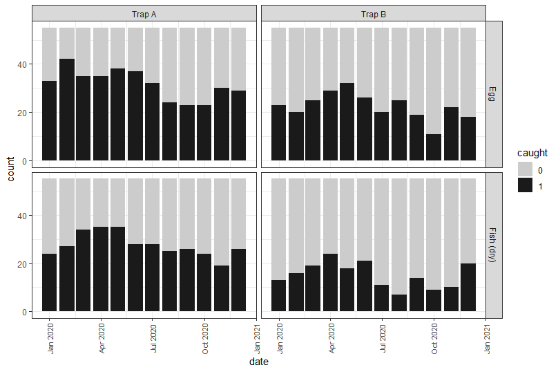
And yeah, there looks to be a pattern with some clear differences between the trap types and bait types. Additionally, it looks a like trap catch could be higher in the first half of the year compared to the second half – but this might just be our imagination.

Now we might try some modelling using glm using model selection (see page 238). Here will use date as as factor:

# setup a subset of models of Table 1
Cand.models <- list( )

# set out of candidate model target

Cand.models[[1]] <- glm(trap.catch ~ bait.type + trap.type + as.factor(date) + cover,
                        data = traps, family = "binomial")
Cand.models[[2]] <- glm(trap.catch ~ bait.type + trap.type + as.factor(date),
                        data = traps, family = "binomial")
Cand.models[[3]] <- glm(trap.catch ~ trap.type + as.factor(date),
                        data = traps, family = "binomial")
Cand.models[[4]] <- glm(trap.catch ~ bait.type + as.factor(date),
                        data = traps, family = "binomial")
Cand.models[[5]] <- glm(trap.catch ~ bait.type ,
                        data = traps, family = "binomial")
Cand.models[[6]] <- glm(trap.catch ~ trap.type ,
                        data = traps, family = "binomial")
Cand.models[[7]] <- glm(trap.catch ~ bait.type + trap.type,
                        data = traps, family = "binomial")
Cand.models[[8]] <- glm(trap.catch ~ cover,
                        data = traps, family = "binomial")
Cand.models[[9]] <- glm(trap.catch ~ 1 ,
                        data = traps, family = "binomial")



# create a vector of names to trace back models in set
Modnames <- paste("mod", 1:length(Cand.models), sep = " ")

# AIC table to 4 digits
aictab(cand.set = Cand.models, modnames = Modnames, sort = TRUE)

Now for the sake of brevity I will skip the disgnostics and look at the predictions made by the top model using the fitted() function. I’ve made a copy of the original traps data now called our.model so that i can attached the predictions without altering the original data set:

our.model <- traps
our.model$prediction <- fitted(Cand.models[[2]])

Now we can graph the predictions to understand the pattern being predicted:

ggplot()+
  geom_point(data = our.model, 
             aes(x = as.Date(date), 
                 y = prediction, colour = bait.type,
                 shape = trap.type), size = 4)+
  geom_smooth(data = our.model, 
              aes(x = as.Date(date), 
                  y = prediction, colour = bait.type,
                  shape = trap.type), fill = NA) +
  theme_bw()+
  xlab("Date")+
  ylab("Predicted probability of catching moongoose")

Which results in:

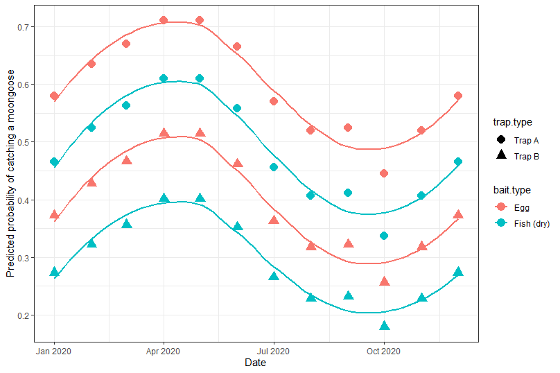
Clearly there seems to be a strong seasonal pattern with differences between the bait and trap types.

BACK to INDEX